把所有的东西集中在一起

管道流

我们已经看到一些估计器可以进行数据转换，一些估计器可以预测变量。我们还可以创建组合估计器同时完成上述任务：

import numpy as np
import matplotlib.pyplot as plt
import pandas as pd

from sklearn import datasets
from sklearn.decomposition import PCA
from sklearn.linear_model import LogisticRegression
from sklearn.pipeline import Pipeline
from sklearn.model_selection import GridSearchCV
# 定义一个管道来搜索PCA截断和分类器正则化的最佳组合。
pca = PCA()
# 将tolerance设置为较大的值加快示例运行
ogistic = LogisticRegression(max_iter=10000, tol=0.1)
pipe = Pipeline(steps=[('pca', pca), ('logistic', logistic)])
X_digits, y_digits = datasets.load_digits(return_X_y=True)

# 可以使用“ __”分隔的参数名称来设置管道的参数：
param_grid = {
    'pca__n_components': [5, 15, 30, 45, 64],
    'logistic__C': np.logspace(-4, 4, 4),
}
search = GridSearchCV(pipe, param_grid, n_jobs=-1)
search.fit(X_digits, y_digits)
print("Best parameter (CV score=%0.3f):" % search.best_score_)
print(search.best_params_)

# 绘制PCA频谱
pca.fit(X_digits)

fig, (ax0, ax1) = plt.subplots(nrows=2, sharex=True, figsize=(6, 6))
ax0.plot(np.arange(1, pca.n_components_ + 1),
         pca.explained_variance_ratio_, '+', linewidth=2)
ax0.set_ylabel('PCA explained variance ratio')

ax0.axvline(search.best_estimator_.named_steps['pca'].n_components,
            linestyle=':', label='n_components chosen')
ax0.legend(prop=dict(size=12))

使用特征脸进行人脸识别

本示例中使用的数据集是“Labeled Faces in the Wild”（也称为LFW）的预处理摘录

http://vis-www.cs.umass.edu/lfw/lfw-funneled.tgz (233MB)

"""
===================================================
使用特征脸和支持向量机的人脸识别示例
===================================================

本例中使用的数据集是“Labeled Faces in the Wild”的预处理摘录，也称为LFW_:

  http://vis-www.cs.umass.edu/lfw/lfw-funneled.tgz (233MB)

.. _LFW: http://vis-www.cs.umass.edu/lfw/

数据集中最具代表性的前5名人员的预期结果:

================== ============ ======= ========== =======
                   precision    recall  f1-score   support
================== ============ ======= ========== =======
     Ariel Sharon       0.67      0.92      0.77        13
     Colin Powell       0.75      0.78      0.76        60
  Donald Rumsfeld       0.78      0.67      0.72        27
    George W Bush       0.86      0.86      0.86       146
Gerhard Schroeder       0.76      0.76      0.76        25
      Hugo Chavez       0.67      0.67      0.67        15
       Tony Blair       0.81      0.69      0.75        36

      avg / total       0.80      0.80      0.80       322
================== ============ ======= ========== =======

"""
from time import time
import logging
import matplotlib.pyplot as plt

from sklearn.model_selection import train_test_split
from sklearn.model_selection import GridSearchCV
from sklearn.datasets import fetch_lfw_people
from sklearn.metrics import classification_report
from sklearn.metrics import confusion_matrix
from sklearn.decomposition import PCA
from sklearn.svm import SVC
print(__doc__)
# 在stdout(标准输出)上显示进度日志
logging.basicConfig(level=logging.INFO, format='%(asctime)s %(message)s')
# #############################################################################
# 下载数据（如果尚未存储在磁盘上）并将其作为numpy数组加载
lfw_people = fetch_lfw_people(min_faces_per_person=70, resize=0.4)

# 获取图像维度（用于绘图）
n_samples, h, w = lfw_people.images.shape

# 对于机器学习，我们直接使用2个数据（因为该模型忽略了相对像素位置信息）
X = lfw_people.data
n_features = X.shape[1]

# 要预测的标签是此人的id值
y = lfw_people.target
target_names = lfw_people.target_names
n_classes = target_names.shape[0]

print("Total dataset size:")
print("n_samples: %d" % n_samples)
print("n_features: %d" % n_features)
print("n_classes: %d" % n_classes)
# #############################################################################
# 使用分层采样交叉切分(stratified k fold)将原始数据集分成训练集和测试集
# 分成训练集和测试集
X_train, X_test, y_train, y_test = train_test_split(
X, y, test_size=0.25, random_state=42)
#############################################################################
# 在人脸数据集（视为未标记数据集）上计算PCA（特征脸）：无监督特征提取/降维
n_components = 150
print("Extracting the top %d eigenfaces from %d faces"
      % (n_components, X_train.shape[0]))
t0 = time()
pca = PCA(n_components=n_components, svd_solver='randomized',
          whiten=True).fit(X_train)
print("done in %0.3fs" % (time() - t0))

eigenfaces = pca.components_.reshape((n_components, h, w))

print("Projecting the input data on the eigenfaces orthonormal basis")
t0 = time()
X_train_pca = pca.transform(X_train)
X_test_pca = pca.transform(X_test)
print("done in %0.3fs" % (time() - t0))
# #############################################################################
# 训练SVM分类模型
print("Fitting the classifier to the training set")
t0 = time()
param_grid = {'C': [1e3, 5e3, 1e4, 5e4, 1e5],
              'gamma': [0.0001, 0.0005, 0.001, 0.005, 0.01, 0.1], }
clf = GridSearchCV(
    SVC(kernel='rbf', class_weight='balanced'), param_grid
)
clf = clf.fit(X_train_pca, y_train)
print("done in %0.3fs" % (time() - t0))
print("Best estimator found by grid search:")
print(clf.best_estimator_)
# #############################################################################
# 测试集上进行模型性能的定性评估
print("Predicting people's names on the test set")
t0 = time()
y_pred = clf.predict(X_test_pca)
print("done in %0.3fs" % (time() - t0))

print(classification_report(y_test, y_pred, target_names=target_names))
print(confusion_matrix(y_test, y_pred, labels=range(n_classes)))
# #############################################################################
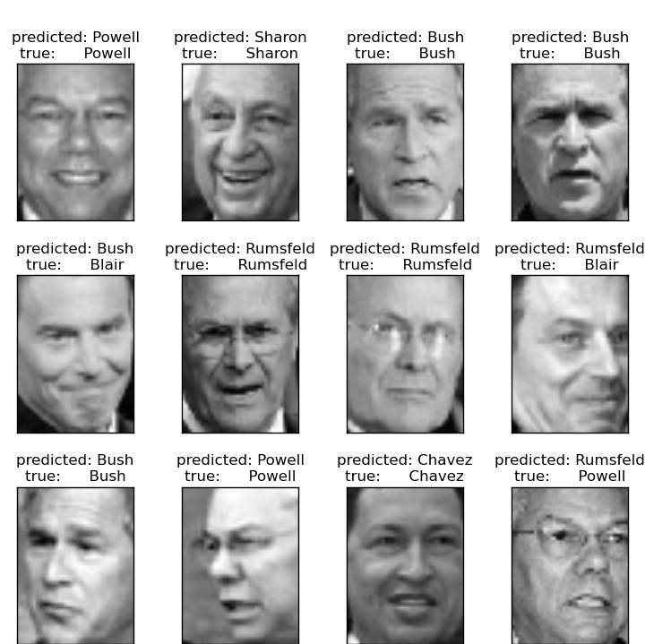
# 使用matplotlib对模型的预测进行定性评估
def plot_gallery(images, titles, h, w, n_row=3, n_col=4):
    """绘制图像的函数"""
    plt.figure(figsize=(1.8 * n_col, 2.4 * n_row))
    plt.subplots_adjust(bottom=0, left=.01, right=.99, top=.90, hspace=.35)
    for i in range(n_row * n_col):
        plt.subplot(n_row, n_col, i + 1)
        plt.imshow(images[i].reshape((h, w)), cmap=plt.cm.gray)
        plt.title(titles[i], size=12)
        plt.xticks(())
        plt.yticks(())
# 绘制部分测试集的预测结果
def title(y_pred, y_test, target_names, i):
    pred_name = target_names[y_pred[i]].rsplit(' ', 1)[-1]
    true_name = target_names[y_test[i]].rsplit(' ', 1)[-1]
    return 'predicted: %s\ntrue:      %s' % (pred_name, true_name)

prediction_titles = [title(y_pred, y_test, target_names, i)
                     for i in range(y_pred.shape[0])]

plot_gallery(X_test, prediction_titles, h, w)

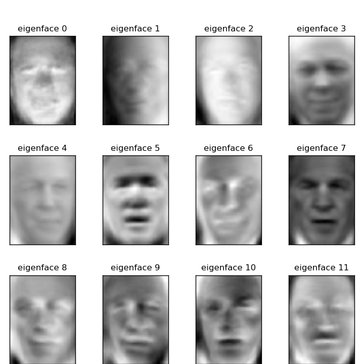
# 绘制最显著的特征脸
eigenface_titles = ["eigenface %d" % i for i in range(eigenfaces.shape[0])]
plot_gallery(eigenfaces, eigenface_titles, h, w)

plt.show()

预测

特征脸

数据集中最具代表性的前5名人员的预期结果：

                   precision    recall  f1-score   support

Gerhard_Schroeder       0.91      0.75      0.82        28
  Donald_Rumsfeld       0.84      0.82      0.83        33
       Tony_Blair       0.65      0.82      0.73        34
     Colin_Powell       0.78      0.88      0.83        58
    George_W_Bush       0.93      0.86      0.90       129

      avg / total       0.86      0.84      0.85       282

开放性问题：股票市场结构

我们能预测在给定的时间范围内谷歌股价的变化吗?

学习图结构